Search - Lecture 0 - CS50's Introduction to Artificial Intelligence with Python 2020


Channel: CS50
Uploaded by CS50 on 20230724
Categories: Education
Tags: cs50, harvard, computer, science, david, j., malan
00:00:00 - Introduction 00:00:15 - Artificial Intelligence 00:03:14 - Search 00:14:17 - Solving Search Problems 00:25:57 - Depth First Search 00:28:30 - Breadth First Search 00:54:29 - Greedy Best-First Search 01:05:15 - A* Search 01:12:01 - Adversarial Search 01:14:09 - Minimax 01:36:17 - Alpha-Beta Pruning 01:45:28 - Depth-Limite

This is a detailed overview of the content of the lecture "Search - Lecture 0 - CS50's Introduction to Artificial Intelligence with Python 2020", presented by Brian Yu.

Overview of the Lecture

This lecture serves as the foundational introduction to AI search algorithms [00:58]. It transitions from classical, single-agent pathfinding problems to more complex adversarial search environments such as board games [01:12:04].

+--------------------------------
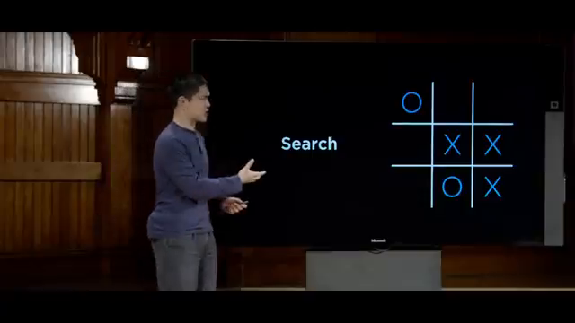
Image for chunk 1

-------+

| Search in AI Lecture |

+---------------------------------------+

|

+-----------------------+-----------------------+

| |

[Classical Search] [Adversarial Search]

- DFS / BFS (Uninformed) - Minimax Algorithm

- Greedy Best-First / A* (Informed)

Image for chunk 2

- Alpha-Beta Pruning

- Depth-Limited Search

1. Foundations of Classical Search

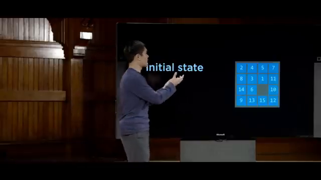
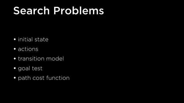
A search problem is defined by an environment where an agent (an entity that perceives and acts) must find a sequence of actions to transition from an initial state to a goal state [04:53].

Core Terminology

State: A configuration of the environment [05:24].

Initial State: Where the agent starts the search [05:53].

Actions: Choices availa

Image for chunk 3

ble in a given state, mathematically represented as a function Actions(s) [06:18].

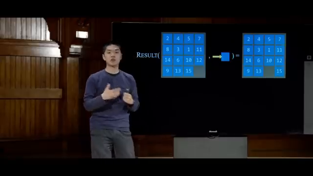
Transition Model: A description of what state results from performing an action in a state, represented as Result(s, a) [07:35].

State Space: The set of all states reachable from the initial state via any sequence of actions [09:29].

Goal Test: A condition to determine whether a given state is a goal state [01:10:04].

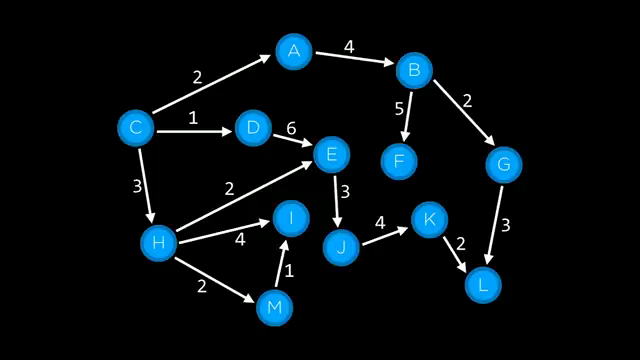
Path Cost: A numerical value assigned to a path representing the resou

Image for chunk 4

rces (time, money, steps) spent [11:55].

Optimal Solution: A solution with the lowest path cost [14:26].

Nodes

To carry out search, computers pack state data into a data structure called a node [15:09]. A node contains:

A state [15:25]

A parent node (for backtracking the final path) [15:30]

The action taken to reach it [16:06]

The path cost [16:11]

2. Uninformed Search Algorithms

Uninformed search strategies use no problem-specific knowledge to make choices [53:12]. Th

Image for chunk 5

ey explore options based purely on the graph structure.

The frontier is the data structure containing all nodes available for exploration that have not yet been visited [16:58].

+-------------------------------------------------+

| General Search Loop |

+-------------------------------------------------+

|

Is the Frontier Empty?

/

Image for chunk 6

\

YES NO

/ \

[No Solution] Remove Node

|

Is it the Goal?

/ \

YES NO

/ \

[Return Path]

Image for chunk 7

Expand Node & Add

Unvisited Neighbors

to Frontier

Depth-First Search (DFS)

Behavior: Explores the deepest node in the frontier first [28:11].

Data Structure: Uses a Stack (Last-In, First-Out) [26:00].

Pros: Can be memory-efficient if a solution is found quickly on a branch [36:06].

Cons: Not guaranteed to find the optimal (shortest) solution and might get stuck in loops

Image for chunk 8

if visited states are not tracked [23:38, 33:31].

Breadth-First Search (BFS)

Behavior: Explores the shallowest node in the frontier first [28:41].

Data Structure: Uses a Queue (First-In, First-Out) [29:02].

Pros: Guaranteed to find the optimal solution [34:49].

Cons: Can be very memory-intensive as it stores many states in the frontier [36:06].

3. Informed Search Algorithms

Informed search strategies use problem-specific knowledge to speed up the search process [53:58]

Image for chunk 9

.

Heuristics

A heuristic function h(n) estimates the cost from node n to the goal [55:21]. In maze problems, a common heuristic is the Manhattan Distance (the sum of horizontal and vertical distances, ignoring obstacles) [56:40].

Greedy Best-First Search (GBFS)

Behavior: Always expands the node that it estimates is closest to the goal according to the heuristic h(n) [54:40].

Limitations: It can make sub-optimal, "greedy" local decisions that lead to longer overall path

Image for chunk 10

s [01:03:20].

A* Search

Behavior: Expands the node with the lowest value of f(n)=g(n)+h(n) [01:05:54].

g(n): The cost to reach node n [01:06:06].

h(n): The estimated heuristic cost from n to the goal [01:06:06].

Optimality Conditions: A* is mathematically guaranteed to be optimal if h(n) is:

Admissible: Never overestimates the true cost to reach the goal [01:09:32].

Consistent: The heuristic value of a node is less than or equal to the cost of stepping to a neighbor pl

Image for chunk 11

us that neighbor's heuristic value [01:10:04].

4. Adversarial Search (Game Playing)

When multiple agents compete with opposite objectives, search becomes adversarial [01:12:04].

MAX Player (e.g., X) -> Tries to Maximize Score

/ | \

/ | \

MIN Player (e.g., O) -> Tries to Minimize Score

/ | \ / | \

[ 1] [ 0] [-1]

Image for chunk 12

[ 0] [-1] [-1] (Terminal Utilities)

The Minimax Algorithm

Minimax models games where two players alternate turns. One player (MAX) tries to maximize the score, while the other (MIN) tries to minimize it [01:16:05].

Terminal Test: Checks if the game is over [01:18:04].

Utility Function: Assigns a numerical value to a terminal state (e.g., +1 for a MAX win, −1 for a MIN win, 0 for a tie) [01:18:36].

Recursive Structure: The MAX player chooses actions assuming the MIN

Image for chunk 13

player will respond optimally to minimize MAX's score, and vice-versa [01:23:38].

Alpha-Beta Pruning

Alpha-Beta Pruning is an optimization that skips evaluating branches in the minimax tree that cannot possibly affect the final decision [01:43:26].

If MAX knows a move guarantees a score of 4, and notices that another path allows MIN to force a score of 3 (or worse), MAX can immediately stop evaluating further actions on that sub-tree [01:41:47].

Depth-Limited Minimax

Image for chunk 14

In games with incredibly vast state spaces (like Chess, which has over 10

120

possible games [01:45:54]), looking all the way to the end is impossible.

Depth-Limited Search evaluates only a set number of moves ahead [01:45:35].

It uses an Evaluation Function to estimate how good a non-terminal state is (e.g., assigning scores based on piece values in Chess) [01:46:26].

Search - Lecture 0 - CS50's Introduction to Artificial Intelligence with Python 2020

CS50 · 958K vie

Image for chunk 15

Viewer Discussion & Comments

@mehuljain5322
the world is being beaten with lockdowns and a virus and yet you guys delivered world class content for free for everyone to learn. LEGENDS!
@aditmagotra6914
This guy talked non stop for 1.5 hours. THANK YOU
@k.h.p.9862
I'm three years late to this 2020 lecture, but never too late to say, "thank you!"
@eugeniar7101
Opened on YouTube just to say THANK YOU for such a detailed and clear explanation!
@MAwaisSEO
this course is not outdated! infact these ai foundations i don't know who else teaches so good